The previous two articles in this series focused on the theory and kernel-level engineering of linear attention. But those discussions were mostly centered on the development environment. In real large-scale deployment, we need many additional optimizations in order to make better use of hardware resources. In this article, I want to discuss linear attention from the perspective of deployment-oriented optimizations, and explain why I believe the infrastructure around linear attention is still in a very early stage.
Quantization
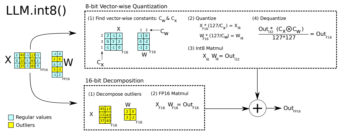
LLM.int8() and Massive Activations
Even before ChatGPT exploded in popularity, some research had already studied the difficulties that full attention architectures face during quantization. In LLM.int8(), the authors point out that some outlier activation values inside full attention can significantly hurt quantization quality, and therefore suggest separating those outliers from the normal values.
This phenomenon is often called Massive Activations. It has been studied extensively, and two major contributing factors are Softmax and RoPE.
Softmax normalization: Softmax enforces the constraint that all attention weights must sum to 1. But in real LLM computation, we often want more flexible behavior. For example, if an input is simple enough that the first 40 layers of a 60-layer model have already done the useful work, then the remaining layers might ideally perform a near no-op, which in a residual network corresponds more closely to outputting 0. To satisfy such requirements, attention may develop behaviors similar to Attention Sink, concentrating attention on irrelevant tokens and producing massive activations.
Recently I have been spending most of my time on inference acceleration, and I also ran a few experiments along the way. This article is meant as the beginning of a short series of notes. I want to start from the perspective of “moving compute” and “moving storage”, and discuss some practical observations around dynamic switching of parallel strategies and KV Cache flow management. In the era of increasingly common Agentic Workflows, can we improve inference efficiency across large clusters by scheduling compute, storage, and bandwidth more intelligently?
Back in the classic big-data era, one interesting question was whether the system should be centered around compute or around data. Over time, the industry settled on the practice of “Move Compute to Data”: SSDs are expensive, IO is expensive, bandwidth is expensive. So instead of moving data around, it is often better to schedule code onto the machine where the data already lives and use the local CPU there. In that world, the scheduler’s core job is to preserve data locality and place computation as close as possible to the disks holding the data.
But in the LLM era, the object we are dealing with is inference for giant models running on GPUs. The thing we would need to move as “compute” has effectively become the model weights themselves, which are huge. In comparison, moving data, that is, moving the KV Cache, starts to look more realistic. But what is actually the right solution?
This article mainly draws on Mamba: The Hard Way and the open-source project flash-linear-attention.
Prefill and Decoding
As we know, Prefill and Decoding are two very different scenarios in attention computation, with the following characteristics:
| Property | Prefill | Decoding |
|---|---|---|
| Input | Long sequence (length $L$) | 1 new token + historical state |
| Common bottleneck | Compute bound (Tensor Core utilization) | Memory / latency bound (state reads/writes + small matrix ops) |
Recall the derivation from the theory article, especially the section on Mamba. Common linear attention variants can usually be written in two equivalent forms:
Matrix form (attention view):
$$ y_i = \sum_{j=0}^i (CausalMask(Q_i K_j^T)) V_j $$
Recurrent form (SSM view):
$$ h_t = A_t h_{t-1} + B_t x_t $$ $$ y_t = C h_t $$
In Decoding, the recurrent form can be used quite directly, so in this article I will focus mainly on how Prefill is implemented.
Common Algorithms for Linear Attention
There are several recurring implementation ideas in linear attention. In this section, I will explain them with reference to flash-linear-attention.
Prefix Scan / Cumsum
Algorithm Overview
Let us first review what Prefix Scan means. In short, Prefix Scan is an optimization technique for associative operators.
Suppose we have $y_t = x_1 ⊗ x_2 ⊗ x_3 … ⊗ x_t$. If $⊗$ is associative, then $y_t$ can be computed efficiently with a reduce-style parallel procedure.
I am planning to write a series of posts about linear attention and use them to organize some of the relevant theory and engineering ideas. This article focuses on the fundamentals.
From Softmax Attention to Linear Attention
Softmax Attention and the $O(N^2)$ Bottleneck
Standard Transformers use softmax attention. Given query, key, and value matrices $Q, K, V \in \mathbb{R}^{N \times d}$, where $N$ is the sequence length and $d$ is the feature dimension, the formula is:
$$ Attention(Q, K, V) = \text{softmax}\left(\frac{QK^T}{\sqrt{d}}\right)V $$
Let us unpack the dimensions step by step:
- Similarity matrix: compute $QK^T$.
- $Q$ has shape $N \times d$ and $K^T$ has shape $d \times N$.
- The result is an $N \times N$ matrix.
- The computational complexity is $O(N^2 d)$.
- Softmax: normalize each row. The shape stays $N \times N$.
- Weighted sum: multiply by $V$.
- An $N \times N$ matrix times an $N \times d$ matrix gives an $N \times d$ output.
- This step is also $O(N^2 d)$.
The core bottleneck is that softmax is nonlinear, so the full $N \times N$ attention matrix must be formed before the weighted sum can happen.
- Compute complexity: $O(N^2 d)$
- Memory usage: $O(N^2)$ if we ignore FlashAttention-like optimizations
- KV cache: during inference we need to keep all keys and values, which costs $O(Nd)$
For a long time this was acceptable, but as agent workloads push context windows longer and longer, the $O(N^2)$ cost is becoming too expensive.
Background
Ever since R1 took off earlier this year, I have seen a lot of discussion about the nature of intelligence. A large part of that discussion seems to converge on one view: language is the foundation of intelligence, and the path to AGI runs through language.
Zhang Xiaojun’s interviews this year with several researchers include two representative examples:
- Yang Zhilin argued that under the current paradigm, multimodal capability often does not improve a model’s “IQ”, and may even harm the language intelligence it already has. In one interview he said that if you want to add multimodal capability, you need to make sure it does not damage the model’s “brain”. At best, multimodality should reuse the intelligence already stored in the text model, instead of creating an entirely separate parameter system that overwrites it.
- Yao Shunyu also emphasized that language seems more fundamental on the road to general intelligence. He originally worked in computer vision, but later concluded that language was the more central and more promising direction. In his view, language is the most important tool humans invented for cognitive generalization, because it forms a closed loop between generation and reasoning.
There are, however, other viewpoints. Some researchers argue that the potential of multimodal capability may be constrained more by the current training paradigm than by multimodality itself. Zhang Xiangyu, for example, pointed out two things:
In the previous article I discussed Ray and the evolution of LLM reinforcement learning frameworks, but I did not really explain why frameworks evolved in that direction instead of starting there from day one. Part of the answer is of course repeated practical optimization, but another equally important part is that the underlying demands of LLM RL also changed.
This article focuses on how algorithms and system frameworks influence each other and co-evolve in LLM reinforcement learning. I will start with two relatively mature case studies, then move on to a few directions that still feel unsettled but, in my view, have a lot of potential.
Typical Cases of Algorithm-System Co-Evolution
Let us begin with two issues where the community already has some degree of consensus.
Case 1: Reasoning Models Driving Disaggregated Architectures
As mentioned in the previous article, earlier RL systems tried to stay as on-policy as possible, so the common design was an on-policy algorithm paired with a colocated architecture. That choice made sense. On the algorithm side, on-policy methods do have sample-efficiency advantages. On the system side, before CoT and test-time scaling became dominant, output lengths were shorter and the compute bubbles caused by inference engines were still tolerable.
LLM reinforcement learning frameworks have been evolving extremely quickly. Ray was one of the frameworks that benefited the most from the ChatGPT wave, and among all stages of LLM training, RL is probably where Ray is used the most. I want to write down the development path of this area and a few of my own views.
Starting from Google Pathways
If we want to discuss Ray and RL systems, a good place to start is Pathways. In 2021 Google proposed Pathways as a next-generation AI architecture and distributed ML platform, and the related work discussed a Single-Controller + MPMD system design in detail.
Single-Controller means using one central coordinator to manage the entire distributed computation flow. There is a master control node responsible for task dispatching, resource scheduling, status monitoring, and orchestration of the whole graph.
Multiple-Controller means using several distributed control nodes that jointly manage different parts of the workload. There is no single global coordinator. Instead, different sub-systems are coordinated through a distributed consistency protocol.
In Ray, the Driver Process is a typical Single-Controller. It can launch and coordinate many different task programs. By contrast, a PyTorch DDP program started via torchrun is a typical Multiple-Controller setup, because each node is running its own copy of the program.
I have been working on Ray Platform for almost two years now and have run into all sorts of issues. I want to write down some of the common pitfalls, starting with Ray Data.
The most common OOM and OOD problems in Ray Data are usually related to backpressure. In fact, the backpressure story here is not just one mechanism. It has several layers:
- Ray Core Generator: controls Ray Generators so that too much data is not produced in the background, which would otherwise cause OOM or OOD.
- Streaming Executor + Resource Allocator:
- controls the output rate of running tasks, so one task does not produce too much data at once
- controls how many tasks a single operator may submit when resources are tight
- Backpressure Policies: additional task-submission rules on top of the core resource checks.
Let us go through them one by one.
Ray Core Generator: Backpressure on Object Count
Ray Generator is similar to a Python generator in that it can be iterated over, but there is one major difference: Ray Generator uses ObjectRefGenerator and continues to run in the background.
That means if one Ray Data read_task is reading a large file, we cannot control its memory footprint just by slowing down downstream consumption. Even if the downstream consumer stops pulling, the task can keep producing new blocks.
I am planning to organize some notes for DeepSeek’s open-source projects, and I also want to refresh my own memory along the way. I will start with FlashMLA.
FlashMLA is DeepSeek’s open-source MLA operator implementation. It is mainly used for inference decoding. Training and prefilling are handled by different kernels.
The figure below gives a rough picture of what the MLA operator computes. I will skip the detailed derivation here. Conceptually, it is a fusion of the following two GEMMs. A few details are worth noting:
- The K and V matrices share part of their parameters.
- The figure only shows the computation for one query head and one KV-head pair. In practice there are also
num_kv_headandbatch_sizedimensions. - There is a softmax between the two GEMMs, but online softmax lets us process it block by block, so it does not change the main computation pattern.

The kernel invocation has two major stages:
- Call
get_mla_metadatato compute metadata that helps optimize kernel execution. - Call
flash_mla_with_kvcacheto do the actual computation.
Before we get into the calls themselves, it helps to look at how FlashMLA partitions the work. This is very similar to FlashDecoding. A single thread block is not required to process an entire sequence. Instead, the runtime uses load balancing to group all sequences together, split them into sequence blocks, and then assign those blocks to thread blocks. The partial results are merged at the end.