Recently I have been spending most of my time on inference acceleration, and I also ran a few experiments along the way. This article is meant as the beginning of a short series of notes. I want to start from the perspective of “moving compute” and “moving storage”, and discuss some practical observations around dynamic switching of parallel strategies and KV Cache flow management. In the era of increasingly common Agentic Workflows, can we improve inference efficiency across large clusters by scheduling compute, storage, and bandwidth more intelligently?
Back in the classic big-data era, one interesting question was whether the system should be centered around compute or around data. Over time, the industry settled on the practice of “Move Compute to Data”: SSDs are expensive, IO is expensive, bandwidth is expensive. So instead of moving data around, it is often better to schedule code onto the machine where the data already lives and use the local CPU there. In that world, the scheduler’s core job is to preserve data locality and place computation as close as possible to the disks holding the data.
But in the LLM era, the object we are dealing with is inference for giant models running on GPUs. The thing we would need to move as “compute” has effectively become the model weights themselves, which are huge. In comparison, moving data, that is, moving the KV Cache, starts to look more realistic. But what is actually the right solution?
1. How Requirements Evolve: From Chat to Agent
System architectures evolve together with the applications they serve.
Phase 1: Single-turn instructions
- Characteristics: the user sends a single instruction, such as translation or summarization, and the model responds. Requests are almost independent of each other.
- Bottleneck: pure compute in Prefill, or memory bandwidth in Decoding.
- Scheduling: simple weighted round-robin is enough. In this phase, KV Cache barely matters. Apart from the system prompt shared by each machine, there is almost no reuse of state, so requests can be scheduled to any node freely.
Phase 2: Multi-turn conversation
- Characteristics: multi-turn conversations can reuse previous context through Prefix Caching. Context gets longer and longer, and each interaction corresponds to one request/response round.
- Bottleneck: GPU memory capacity, which then turns into Prefill time.
- Scheduling: this is when affinity scheduling starts to appear. To maximize cache hits, we try to route the request to the node that already stores that user’s historical context. This is exactly “Move Compute to Data” because recomputing Prefill is too expensive, while moving KV Cache was not yet common at scale. The downside is that hotspots start to appear.
Phase 3: Agentic Workflow
- Characteristics: system prompts, tool definitions, chains of thought, and context can all be shared across parallel branches. Multi-turn conversations can be executed in parallel, but from the user’s perspective the interaction becomes one task completion rather than many back-and-forth turns.
- Bottleneck: the dependency graph becomes far more complicated, and naïvely reusing KV Cache creates severe load imbalance.
- Scheduling challenge: if we keep following “Move Compute to Data”, hotspots become much worse. Nodes containing hot context get overwhelmed, while idle nodes remain useless because they do not hold the data.
As requirements change, we stop looking only at per-request TTFT or TPOT. Instead, we start to care about the completion time of the whole agent task and the overall system throughput.
2. The Core Tradeoff: Moving Compute vs Moving Storage
To resolve the tension in the Agent era, we need to rethink the central tradeoff in scheduling. In the big-data era, moving data was expensive. In the LLM era, the picture is more complicated:
- Moving compute, including moving weights or recompiling computation graphs, is also expensive.
- Compute is gradually overtaking storage as the dominant cost. One storage engineer jokingly said: “We are finally no longer the most expensive part.”
- NVLink and RDMA are making data movement, specifically KV Cache movement, cheaper and cheaper.
For LLM systems, different parallel strategies also lead to different performance tradeoffs, and each strategy fits different request patterns, such as batch size, prompt length, Prefill-heavy workloads, or Decoding-heavy workloads. So in this article I distinguish two kinds of “moving compute”:
- Move compute to a better node that already has the model deployed, such as in PD disaggregation, without moving weights.
- Move compute to a fresh empty node, which is really the classic autoscaling case.
In practice today, I have found the cost of the second type of compute movement to be extremely high even under the constraints of the first. And since we usually want to maximize system utilization, we only treat it as a last resort when the current system cannot handle the task at all. So I will not expand on it here. The rest of the article focuses on the first kind of compute movement and uses it as the cost model for “moving compute”.
That leaves the scheduler with a two-way choice:
| Strategy | A. Prefer nodes with higher compute efficiency (Compute-First) | B. Prefer nodes with higher storage efficiency (Data-First) |
|---|---|---|
| Cost | Must move data (KV Cache transfer consumes bandwidth) | May need to wait for compute (queueing) or run on a suboptimal node |
| Best fit | Bandwidth is plentiful, latency matters, compute is scarce | Bandwidth is tight, throughput matters, compute is plentiful |
| Typical examples | PD disaggregation, hotspot protection | Multi-turn chat with KV Cache reuse |
This tradeoff is not fixed. It depends on several variables:
-
Relative scarcity of compute vs bandwidth
- If GPU compute is extremely tight, such as during peak hours, letting GPUs idle while waiting for cache locality is a huge waste. In that case, strategy A is preferable.
- If cross-node bandwidth is the bottleneck, for example across racks or data centers, then frequent KV Cache movement introduces unacceptable latency. In that case, strategy B becomes preferable.
-
Batching strategy
- Large-batch / throughput-oriented workloads can afford some scheduling delay in order to build better batches, which pushes the system toward B.
- Small-batch / latency-sensitive workloads value every millisecond, so the scheduler needs to find available compute immediately, which pushes the system toward A.
-
Latency vs throughput as the optimization target
3. Shift Parallelism: Moving Compute Inside a Node
Snowflake’s Shift Parallelism is a very elegant design. By rearranging computation ahead of time, in other words by moving compute rather than data, it reduces the runtime cost of moving data to zero.
Traditional inference deployment is usually either TP (Tensor Parallelism, lower latency) or SP / DP (Sequence / Data Parallelism, higher throughput):
- At low load: we prefer TP to reduce latency.
- At high load: we prefer SP to improve throughput.
The core idea of Shift Parallelism is: instead of moving data such as KV Cache, change the computation strategy itself.
Shared Storage: KV Cache Invariance
By carefully analyzing different parallel strategies, Shift Parallelism observes that the memory layout of KV Cache under Ulysses SP is identical to that under classic TP. This means that when the system switches from TP to SP at runtime, KV Cache does not need to be moved or rearranged at all. With careful computation scheduling, the system can avoid touching storage entirely.
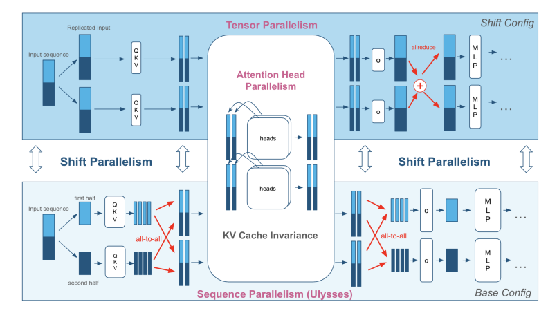
So Shift Parallelism chooses “shared storage”: it pre-arranges the computation such that work can shift from one process to another, improving overall compute efficiency and reducing compute scarcity, without moving the KV Cache.
The tradeoff is that to support seamless switching between TP and SP, the GPU must simultaneously store the different weight layouts needed by both modes.
Some experimental observations:
I also ran a few experiments and analyses based on ArcticInference. In the current implementation, TP and SP effectively keep two copies of the weights. On each GPU, the weights required by SP are actually a superset of those required by TP.
In theory, it might be possible to keep only the SP version of the weights, but the performance cost would be huge. The main issue is the requirement for weight-matrix contiguity in GEMM:
- Compute kernels such as cuBLAS usually require the input tensors to be contiguous in memory. If we try to slice the SP weight matrix directly, that requirement is violated.
- In principle one could write a custom CUDA kernel to handle this more complex non-contiguous mapping, but the engineering cost would be high, and the fragmented memory access pattern would likely destroy coalescing and still lead to poor effective bandwidth.
So Shift Parallelism effectively trades VRAM capacity (redundant weight storage) for compute mobility (dynamic switching between parallel strategies), and thereby avoids expensive runtime data movement.
4. llm-d: Data Flow Across the Cluster
If Shift Parallelism continues the idea of “let compute adapt to the data,” then llm-d argues for the opposite direction: let data move toward compute. As an Agentic Runtime, it treats KV Cache as something that should flow across the cluster.
Breaking the Obsession with Data Locality
As discussed above, Agent workflows are complex and heavily imbalanced. As the entry point to the cluster, llm-d no longer optimizes only the latency of one request. It wants to optimize the end-to-end task completion time.
In the latest community proposals, the system advocates using P2P NVLink or RDMA to move KV Cache quickly between nodes. That allows the scheduler to choose the least loaded or logically closest compute node, rather than staying pinned to the overloaded node that happens to hold the historical cache.
This is reminiscent of how cloud-native databases evolved from “shared nothing” to compute/storage disaggregation or even shared storage/shared memory models. Future inference clusters may well look like a huge shared memory pool interconnected by a high-speed fabric.
Semantic KV Cache
To make such movement efficient, the community argues that llm-d should not blindly move all cache data. The cluster scheduler must understand the Agent workflow and understand the semantic value of KV Cache:
- System prompts / tool definitions: highly reused “static” data -> proactively replicate it to multiple nodes.
- Reasoning branches: transient data that is quickly discarded -> evict with low priority.
This brings us back to the tradeoff: for high-frequency data we replicate to reduce transfer, while for low-frequency data we transfer to better balance compute.
That in turn raises the bar for llm-d scheduling. Replication is no longer a passive reaction when requests arrive. The system needs something closer to instruction prefetching: it has to predict future use and pre-arrange KV Cache ahead of time so that the needed cache is already available where the computation will run.
5. Looking Forward: Reconstructing the Space-Time Model of Inference Systems
If we combine these two directions of thought, future inference systems may have the following characteristics:
-
Hierarchical flexibility
- Inside one node: techniques like Shift Parallelism keep KV Cache fixed while dynamically adjusting the computation graph, such as switching between TP and SP, in order to trade latency against throughput.
- At the cluster level: semantic KV Cache plus P2P interconnects allow the system to proactively move KV Cache and balance load across nodes.
-
KV Cache evolves from “static cache” into “flowing data” It is no longer just a passive cache waiting to be hit. It becomes a first-class resource managed by the scheduler. It may live as static replicated state, or it may move dynamically according to workload demand.
-
Intelligent scheduling and traffic shaping Future scheduling will not stop at passively forwarding traffic. It will actively participate in data aggregation and KV Cache movement so that different classes of workload overlap better in time and avoid contention, thereby amortizing unavoidable costs.
-
The cost of computational context, and exchanging space for time Whether it is redundant weights in Shift Parallelism or proactively replicated context in llm-d, both point to the same underlying idea: weights and context are both part of the computational context.
- Reconstructing that context at runtime, whether by repartitioning weights or recomputing context, is extremely expensive. It consumes SMs and may force CUDA graph recompilation.
- Therefore, exchanging space for time will become normal. Even though VRAM is expensive, we will still be willing to pay that storage tax to gain better compute mobility.
Finally, it is worth briefly mentioning Baidu’s latest work, such as SPS. The strategy proposed there is no longer just real-time traffic forwarding. Instead, it reshapes traffic based on load awareness: the scheduler can buffer requests locally and release them together only when the right conditions are met, actively molding the workload into the form that best matches the current system state. In a sense, that pushes dynamic batching up from the model server into the gateway or scheduler layer.
Following this direction, the boundary between the inference system and the scheduling service will become increasingly blurry. The two schedulers, one at the gateway and one inside the inference engine, will become more tightly coupled. Scheduling itself will shift from passively handling requests to actively managing both compute and data: shaping traffic upstream with batching, matching compute shape with dynamic parallel strategy switching in the middle, and coordinating storage shape downstream through KV Cache flow and replication.
Inference acceleration seems to be moving away from pure kernel optimization and toward full-system orchestration. At the core of that transition is still the movement of compute and storage. Once we add multimodality, sparse attention, linear attention, Engram, and other architectural changes on top, the system we end up with may look less like a simple two-layer service of “gateway -> inference engine” and more like one huge inference cluster.
In short, there is still a great deal left to explore in 2026.
Last modified on 2026-01-29